
On a cold afternoon, standing on a bluff above 907F and her Junction Butte packmates, I could hear the wind cross the ridge before I saw it. It slid through the timber, rattled last year’s leaves, and pulled at my coat. If you listen long enough, you begin to notice the spaces between gusts. And, as a linguist, I thought of the pattern underneath the wind.
What you don’t see is the dance of the molecules, millions of them, colliding and ricocheting in all directions. One molecule hits another close by, which hits another farther away, and in this way a movement in one place ripples invisibly into motion somewhere else. Language is like that. Each word is a molecule in a larger current, seemingly disconnected from distant words, yet bound to them through invisible chains of relationship.
Our words are part of an invisible map, laid out in the brain like trails on a mountainside. Every trail connects to others. You can go from wolf to howl to moon in a few steps, and the path makes sense. We can link thousands of such trails and cross the map any way we choose. That is why I can say The wolf howled under the moon because it missed its pack, and you can follow me there.
Other animals have words too, if a word is a signal that points at something in the world. A Gunnison’s prairie dog’s alarm call differs for a hawk, a coyote, a dog and a person. A bottlenose dolphin invents a whistle that means itself, and its companions copy the whistle to call it by name. Wolves have a repertoire of roughly a dozen graded calls, from whine and whimper through bark and growl to the howl, and howls alone come in enough variants that one study sorted the howls of thirteen wild canids into twenty-one types. These are words in the sense that they point. But they live on smaller maps. A few trails. A handful of landmarks. That is why context matters so much when we try to understand what a wolf means.
A few animals have carried words across the species line. A border collie named Chaser learned to recognize the names of more than a thousand objects. Alex, an African gray parrot, used about a hundred spoken labels and could sort things by color, shape and number. Kanzi, a bonobo who died in 2025, used a few hundred keyboard symbols and responded correctly to most of 660 novel spoken sentences. Koko the gorilla’s famous thousand signs were never independently verified. And in 2024, researchers analyzed 194,901 button presses by 152 pet dogs using FluentPet soundboards: 29 percent of the presses were two-button combinations, and some pairs, such as food and play, came up more often than chance or copying the owner could explain. The authors were careful: the study says nothing about what the dogs mean, and nothing about grammar.
What none of these animals has done is combine their words into long, endlessly varied sentences.
Somewhere in our deep past, our brains crossed a line. Our vocabularies swelled, our connections multiplied, and the trails joined into a network so dense that you could walk it forever without retracing your steps. When I first wrote this page, I put that line at about 250 words, the point in a child’s second year where I imagined the word network “percolating” into one connected whole. That was my working assumption. I have since taken it to the data, and the rest of this page is what I found. The short version: the line is real, but it is not a count.
Inside the skull, this map is not built in one place. The brain’s language network lives mostly in the left frontal and temporal lobes, with language-responsive sites beyond it, in the cerebellum, the hippocampus and elsewhere, whose jobs are still being worked out. Work by Evelina Fedorenko and colleagues shows that these language circuits are separate from the systems we use for reasoning and other kinds of thought: people who lose language to a stroke can still do arithmetic, follow music and read other minds.
Artificial intelligence language models work in a related way, though they are made of code, not neurons. They place every word, phrase and sentence as a point in a vast cloud, and the geometry of that cloud, its distances, directions and clusters, encodes meaning. Think of constellations: each star is a word, and their positions relative to each other tell you which belong to the same figure. In 2024, Ariel Goldstein and colleagues recorded from the brains of three epilepsy patients while they listened to a story and found that the word-by-word activity in one language area lined up with the geometry of GPT-2’s word vectors closely enough that a word held out from the fitting could be located in brain-activity space from its neighbors. Both brain and machine can place a point they have not visited by knowing the shape of the space around it.
That is what “geometry” means here: the pattern of relationships. In a map of peaks, the distances and directions between points tell you where the next ridge lies; in a semantic map, the angle between wolf, howl and moon can tell you where night probably sits. Brains and machines both use these relationships to predict what should come next and to weave meaning from context.
The distinction between the machinery for language and the machinery for thought matters here. Thought is not locked inside language. About one in four patients who appear completely unresponsive after a severe brain injury show brain activity in response to spoken commands. The machinery for thought can run without the machinery for speech. And if that can be true for us, silent but thinking, then perhaps it is true for the elk in the meadow, the raven in the wind, or the wolf on the ridge. They may not have our kind of words, but they may have their own mountains of thought. If we accept that, we might choose to treat them as fellow travelers through their own unseen maps.
What is measured: how children get from words to sentences
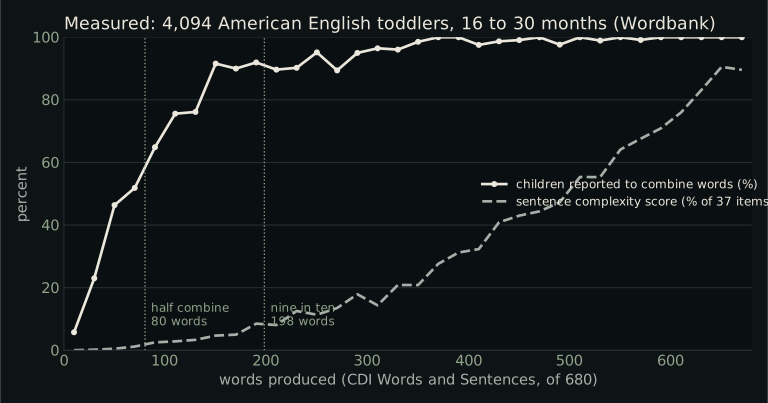
The best record of early vocabulary is the MacArthur-Bates Communicative Development Inventory, a checklist parents fill in. Wordbank, an open archive run by Michael Frank and colleagues at Stanford, holds tens of thousands of these checklists. For American English, the toddler form lists 680 words and also asks whether the child has begun to combine words and which of 37 sentence pairs sounds more like the child.
The numbers people repeat are half right. By 24 months the median American English toddler is reported to say about 300 of the 680 words. “About 50 words at 18 months” is too low as a median; the median 18-month-old is closer to 70 to 85, and reaches 50 words somewhere between 16 and 20 months. More important than either figure is the spread. At 24 months, one child in ten says fewer than about 70 words and one in ten says more than about 550.
The “vocabulary spurt” is less solid than its reputation. When researchers test child by child for a sudden change in the rate of learning, they find it in a minority, five of 38 children in one careful study. Most children simply accelerate, and Bob McMurray showed in 2007 that acceleration is what you expect when many words are being learned at once and most of them are hard. Paul Bloom’s book, often cited for the spurt, argues that the spurt as a transition does not exist.
Grammar, on the other hand, tracks vocabulary very closely, more closely than it tracks age. Elizabeth Bates and her colleagues called this the “critical mass” idea in the 1990s, and the Wordbank data confirm the shape they described: a smooth, accelerating curve. We checked it ourselves on 4,094 checklists. Half of children are reported to combine words by the time they say about 80 words (95 percent interval 75 to 85), and nine in ten by about 200 words (182 to 214). Sentence complexity rises as a smooth function of vocabulary, reaching about a tenth of its maximum at 200 to 250 words and climbing steeply above 400. We fitted a model with a sharp break and models without one; the smooth models fit better. There is no step at 250 words, or at any other number.
What is modeled: when a network of words connects
Network scientists have a precise version of my picture of trails joining into a map. Make each word a node, draw a link between words that are related, and ask how big the largest connected piece is, the “giant component.” In a randomly wired network, Paul Erdős and Alfréd Rényi showed in 1960, the giant component appears once the average node has more than one link, and its share of the network solves a simple equation, S = 1 - e^(-cS), where c is the mean number of links per node. The change is continuous: a slope, not a cliff. On a network of a few hundred words it is a gentle slope.
Two things follow that I did not appreciate when I first drew my graphs. First, the threshold is in links per word, not in the number of words. A growing network with a fixed rule for drawing links will always connect at some size, and that size is set by the rule. Second, a network built from word meanings is a geometric network: words are points in a space, and a link means two points are close. Such networks need more than one link per node to connect, and the number depends on the shape of the space.
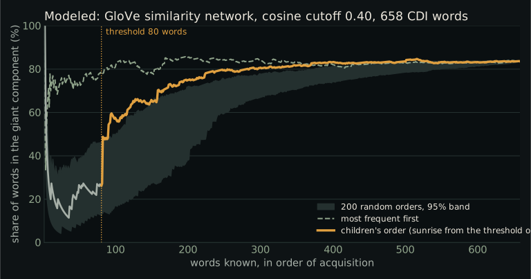
We built the network honestly to see what it does. The words are the 658 checklist words that have a fixed form. Their meanings come from GloVe, a set of word vectors trained on Wikipedia and newswire and released into the public domain; two words are linked when the cosine of the angle between their vectors is at least a cutoff. The words are added in the order American English toddlers typically learn them, estimated from 9,537 Wordbank checklists, and after each word we record the giant component. Against that we grew the same network in 200 random orders and in most-frequent-first order.
At a cutoff of 0.40, the network grown in children’s order passes its threshold at 80 words, where random orders need about 150 (95 percent band 59 to 274). Children learn well-connected words first, a pattern Thomas Hills and colleagues named “preferential acquisition,” and the percolation curve shows it: the children’s map connects early. That 80 happens to match the vocabulary at which half of children combine words. It is a coincidence of the cutoff, and I want to be plain about that, because the threshold moves when the cutoff moves: 61 words at 0.35, 80 at 0.40, 223 at 0.45, 225 at 0.50. My old number, 250, is what this network does at a strict cutoff. What stays put across cutoffs is the mean number of links per word at the threshold, between 1.5 and 2.6, which is what the mathematics predicts for a geometric network.
We also built a second network from a different kind of link: not words that mean similar things, but words that adults actually say next to each other when talking to children, taken from 765,817 adult utterances to children under three in the CHILDES corpora. This “said together” network is dense and connected from the first few dozen words in any order. The supply of two-word frames a child could fill grows roughly with the square of the vocabulary: about 700 attested frames at 150 words, nearly 14,000 at 658. Whatever paces the move from words to sentences, it is not a shortage of linked words.
What the data suggest instead: connectors, not counts
If size is not the line, what is? We asked a sharper question of the same 4,090 children: holding vocabulary size fixed, does the structure of a child’s own words predict whether they combine?
Similarity structure does not. How connected a child’s words are in the meaning network adds nothing once you know how many words they have. But the “said together” structure does, strongly and at every vocabulary size: two children with the same number of words differ in their odds of combining according to how many of their words sit in adult two-word frames. And the words that carry the effect are the small ones. Counting a child’s function words, the more, no, up, mine, in, want that glue phrases together, improves the prediction of combining beyond vocabulary size, while counting verbs or adjectives does not.
This is a first pass on cross-sectional parent-report data, not a peer-reviewed finding, and it has limits we describe in the notes. But it reframes my hypothesis in a way that can be tested. A vocabulary becomes generative not when it reaches a count but when it contains the connectors. The one developmental phase transition that has been measured in children’s own speech points the same way: Bernat Corominas-Murtra and colleagues built networks from a child’s own utterances and found a sharp change from tree-like to small-world structure between about 24 and 28 months, at the moment utterances passed two words, with function words such as a and the taking over as hubs.
Why humans, and not the wolf
Theory offers a cleaner answer than a word count to the question of why only we combine without limit. Martin Nowak and colleagues showed in 2000 that in a population learning its signals by exposure, syntax, separate words for things and for actions, combined, pays off only when the number of events worth talking about exceeds a threshold set by how much harder the combined signals are to learn. In their worked example the crossover comes at about 18 nouns and 18 verbs covering more than a hundred events. The threshold is in the ratio of meanings to signals, not in the number of signals. Simon Kirby’s laboratory languages make the same point from the other side: compositional structure appears when learners see only part of a large meaning space and still have to communicate.
Thom Scott-Phillips and Richard Blythe went further in 2013 and argued that having many signals is not even the right variable. Primates have large gesture repertoires and do not combine them; putty-nosed monkeys have a tiny repertoire and do. In their model a combined signal can evolve only when the combination is already informative on its own, and a separate holistic call would not do the job. Humans escape the constraint because our communication is ostensive: a child who points at a jar and makes a twisting gesture has made a new combination, understood from the moment it is produced, because we read intentions.
The animal record fits. A handful of wild species combine two or three calls into meaning: Japanese tits, pied babblers, Campbell’s and putty-nosed monkeys, chimpanzees, and, in a 2025 study of 700 utterances, wild bonobos, whose seven call types enter four compositional structures. Nightingales sing hundreds of distinct song types and none of them means anything on its own. Repertoire size predicts neither. Whether any of this should be called syntax is itself disputed; the combinations are small, fixed and mostly two elements long.
So the wolf, with a dozen graded calls, a social life conducted largely through scent, posture and presence, and a howl that carries for miles, is what the theory predicts. Whether a wolf’s things worth saying ever outnumber its calls is an empirical question, and it is one that recordings like ours can, in principle, bear on.
Notes on the data
The checklist data are from Wordbank (CC BY 4.0), American English Words and Sentences form, ages 16 to 30 months: the public child-by-word release (version 3.3, 10,173 children) for ages of acquisition, and the Wordbank book’s cache for the per-child analyses (5,520 children; 4,094 with the combining item). Word vectors are GloVe 6B, 300 dimensions (public domain). The “said together” network uses adult speech to children aged 0 to 36 months in 37 American English CHILDES corpora (765,817 utterances; CC BY-NC-SA 3.0), linking words said adjacently at least five times and more often than chance. Thresholds are the vocabulary size at the peak of the second-largest component, the standard finite-size estimate. Our analyses are cross-sectional, rest on parent report, cover one language, and are not peer reviewed; the scripts, outputs and a full account of what the literature does and does not support are in the project’s research notes.